Data - Variable Definitions and Pre-Selection Cuts

Introduction

The variables (features) comprising a HEP analysis dataset are physical observables measured by a (particle) detector. These quantities characterize the physical phenomena studied in the context of a HEP experiment. Different experiments might be interested in measuring different observables. For example, some frequently measured quantities are the transverse momentum of the particles with respect to the particle beam axis, the total energy measured in the event, and the angles between the momenta of different particles; this list is by far exhaustive of what can and has been measured.

In contrast with their diversity, all these variables follow probability distribution functions which can be computed via a combination of analytical methods and numerical Monte Carlo simulations. However, the real physical features are not identical to the ones predicted by the theoretical simulation. The measured distributions are distorted by the finite resolution and limited acceptance of the detectors, among other subtle effects such as errors in the read-out electronics. Thus, the overall detector effects are taken into account via complex simulations that model the interaction of the produced particles with the different components of the detector. This process aligns the measured distributions with the theoretical expectation, up to some technically irreducible uncertainties. Specifically, in the $t\overline{t}H(b\overline{b})$ study, Monte Carlo (MC) data samples were generated by using Powheg v.2 [1-3] for hard scattering computations, Pythia 8 [4] for parton shower simulations and Delphes v.3.4.1 [5] for a fast and simplified detector response simulation.

Current physics analyses investigating the $t\overline{t}H(b\overline{b})$ process are using analytic methods such as the Matrix-Element Method [6], as well as Boosted Decision Trees (BDTs) and Neural Networks (NN) to tackle the discrimination of the signal over the overwhelming background [7,8]. The inputs of these ML models are called feature vectors. Thus, in HEP, the elements of the feature vectors are the physical observables. The physical observables used in the $t\overline{t}H(b\overline{b})$ analysis are defined below.

Definitions

The four-momentum of an analysis object – e.g. reconstructed particle or jet — can be written as

\[\begin{equation} p^{\mu} = \begin{pmatrix} E\\p\sin\theta\cos\phi\\p\sin\theta\sin\phi\\p\cos\theta \end{pmatrix} =\begin{pmatrix} E\\p_x\\p_y\\p_z \end{pmatrix}=\begin{pmatrix} m_T\cosh y\\p_T\cos\phi\\p_T\sin\phi\\m_T\sinh y \end{pmatrix} \end{equation}\]

where Greek indices enumerate the space time coordinates $0,1,2,3$ and the Einstein summation convention is implied.In the first expression the four-momentum is expressed in spherical coordinates and in the second equality in Cartesian coordinates. Finally, $p^\mu$ is represented in the ($p_T,y,\phi$) coordinate system that is conventionally used in HEP. The transverse momentum $p_T$ and mass $m_T$ are defined as

\[\begin{equation} p_{T}\equiv p_\perp=\sqrt{p_x^2+p_y^2}=p\sin\theta\quad\text{and}\quad m_T=\sqrt{p_T^2+m^2} \end{equation}\]

The angle $\phi$ is that of the transverse plane (the plane that is perpendicular to the accelerator beam axis, conventionally chosen to be the z-axis of the coordinate system) and $y$ is the rapidity.

The rapidity variable is useful but non-trivial. To understand it, one starts at the Lorentz transformation along a direction, which can be always picked to be the z-axis:

\[\begin{equation} p'^\mu=\Lambda^\mu_{\nu}p^\nu\Rightarrow \begin{pmatrix} E'\\p_z' \end{pmatrix} =\begin{pmatrix} \gamma & -\gamma \beta\\ -\gamma\beta &\gamma \end{pmatrix} \begin{pmatrix} E\\p_z \end{pmatrix}. \end{equation}\]

The lorentz transformation can be equivalently written as a hyperbolic rotation

\[\begin{equation} \begin{pmatrix} E'\\p_z' \end{pmatrix} =\begin{pmatrix} \cosh y & -\sinh y\\ -\sinh y & \cosh y \end{pmatrix} \begin{pmatrix} E\\p_z \end{pmatrix}, \end{equation}\]

where the relations

\[\begin{equation} \tanh y=\beta,\, \cosh y=\gamma,\, \sinh y=\gamma\beta \label{eq:rapitity_beta_relation} \end{equation}\]

have been imposed. Using the identity

\[\begin{equation} \text{arctanh}x=\frac{1}{2}\log\left(\frac{1+x}{1-x}\right) \end{equation}\]

the rapidity is defined as

\[\begin{equation} y=\text{arctanh}\beta=\text{arctanh}\left(\frac{p_z}{E}\right)=\frac{1}{2}\log\left(\frac{E+p_z}{E-p_z}\right). \end{equation}\]

Furthermore, the pseudo-rapidity is defined by taking the massless particle limit $m\to 0$ of $y$. Thus, for a massless particle

\[\begin{equation} \eta\equiv \lim_{m\to0}y=\lim_{m\to0}\log\left(\frac{E+p\cos\theta}{E-p\cos\theta}\right)=-\log\tan\left(\frac{\theta}{2}\right) \end{equation}\]

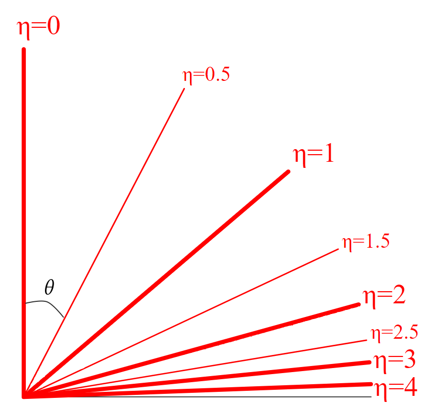
^{Pseudorapidity as a function of the angle $\theta$ ($\eta(\theta=0)=0$).}

The coordinate system $(p_T,y,\phi)$ or more often $(p_T,\eta,\phi)$, has convenient properties. Namely the $p_T$ and $\phi$ are relativistically invariant under Lorentz transformations (boosts) along the z-axis. Additionally, the rapidity and pseudo-rapidity have the additive property under a Lorentz boost, e.g. along the z direction:

\[\begin{equation} \eta \xrightarrow{\text{Lorentz boost}} \eta + \xi \end{equation}\]

where $\xi$ is the pseudo-rapidity parametrising the Lorentz boost (same also holds for rapidity). This property means that differences $\Delta\eta$, between the rapidity of different particles or objects in general, are invariant under z-boosts. The pseudo-rapidity can be expressed in terms of the azimuthal angle $\theta$ and thuss $\Delta\eta$ between two particles carries information about the differences between the angular distributions of their momenta.

A metric in $(\phi,\eta)$ space can be defined, motivated by the aforementioned properties

\[\begin{equation} \Delta R = \sqrt{\Delta\eta^2 + \Delta\phi^2}. \end{equation}\]

This metric is a relativistically invariant way of quantifying the difference between the momentum directions of two reconstructed particles or jets.

Particles that interact weakly with matter such as neutrinos or potential beyond the standard model particles cannot be detected using the detectors of the LHC experiments. Nevertheless, one can indirectly probe their production by defining the missing transverse momentum (MET) and missing transverse energy

\[\begin{aligned} &\vec{\not{p}}_T=-\sum_{\text{observed}} \vec{p}_T\\ &\not{E}_T=|\vec{\not{p}}_T|,\;\text{for a massless non-detectable particle} \end{aligned}\]

The transverse instead of the full momentum is used because the total transverse momentum of every event is zero, since the initial colliding protons have momentum only along the z-axis (beam axis). This means that if we sum the transverse momentum of all the reconstructed objects it should add up to zero. Of course, to conclude that MET is coming from an undetected particle, like a neutrino, with a certain statistical confidence level, other effects need to be investigated, such as systematic uncertainties in the $p_T$ reconstruction algorithms, detector effects etc. If it does not, then the missing transverse momentum and energy is a signature of an undetected particle.

On the contrary, we do not know in every collision the momentum along the beam axis of the colliding particles a priori. That depends on the initial $p_z$ momenta of the partons that constitute the accelerated protons and have a fraction of its momentum and energy. These fractions are random variables that follow the parton distribution functions. Thus, it is clear that we do not have access to this initial condition of $p_z$ for every event and subsequently we do not know the total $\vec{p}$ of an event, to which the reconstructed analysis objects should add up to.

Finally, let us introduce the b-tag variable. Jets are reconstructed from collimated particles. The jet object has a four-momentum given by the sum of it’s constituents, which are identified with dedicated algorithms such the AK4 [9]. Typically in such algorithms, jets are represented as a collection of particles within a cone defined by a radius in terms of the $\Delta R$ distance (see Eq. 10).

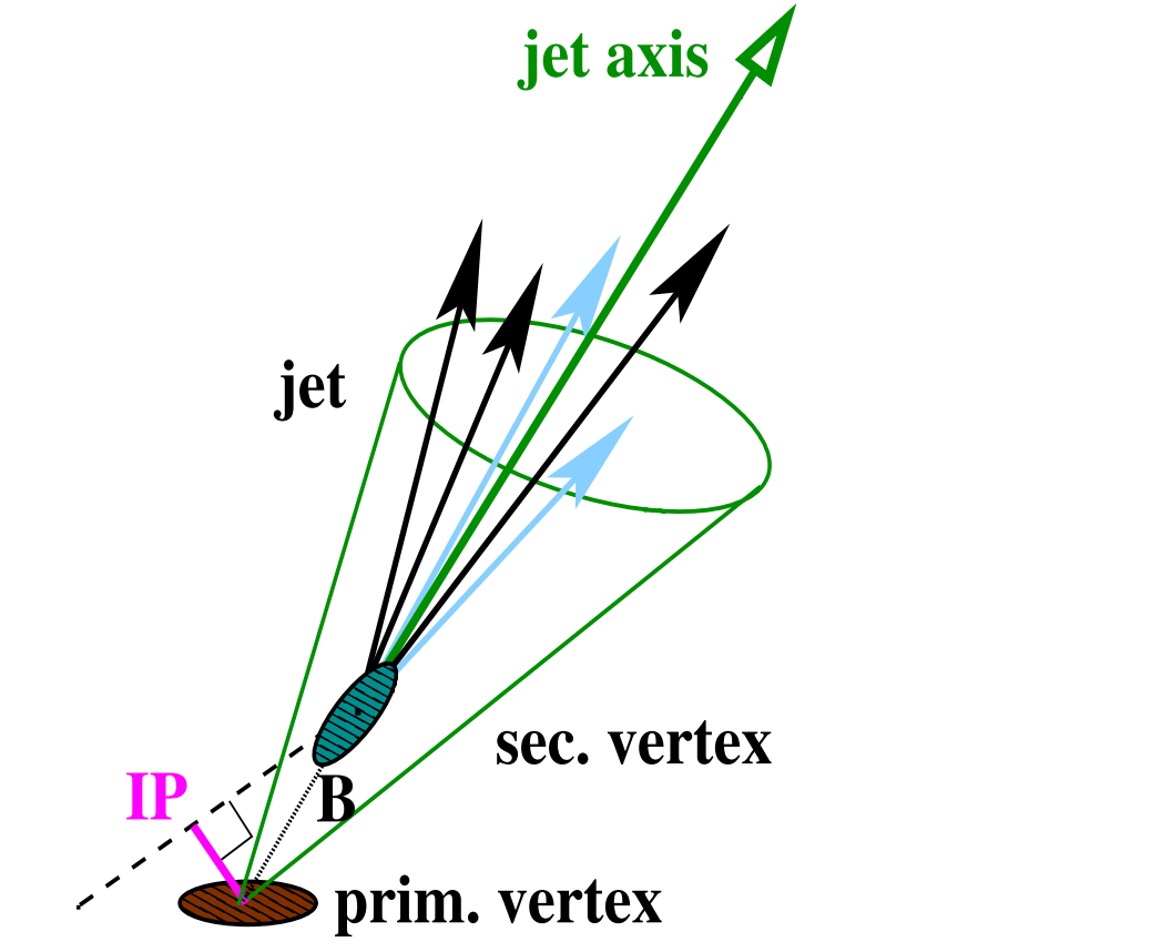
^{Reconstruction of a b-jet. The jet axis is defined by the sum of the particle momenta inside the cone. The primary and secondary vertices are depicted. The former is from the hard-interaction point and the latter from the decay of a B hadron.}

For the jets produced by heavy $b$ and $c$ quarks, further algorithms have been developed which can flag, or tag, i.e., identify their flavour. For instance, the b-tagging algorithms check if the jet is originating from a secondary vertex, its shape, substructure, energy and momentum distributions. Moreover, apart from physics inspired criteria a combination of ML models is also utilized for b-tagging tasks.

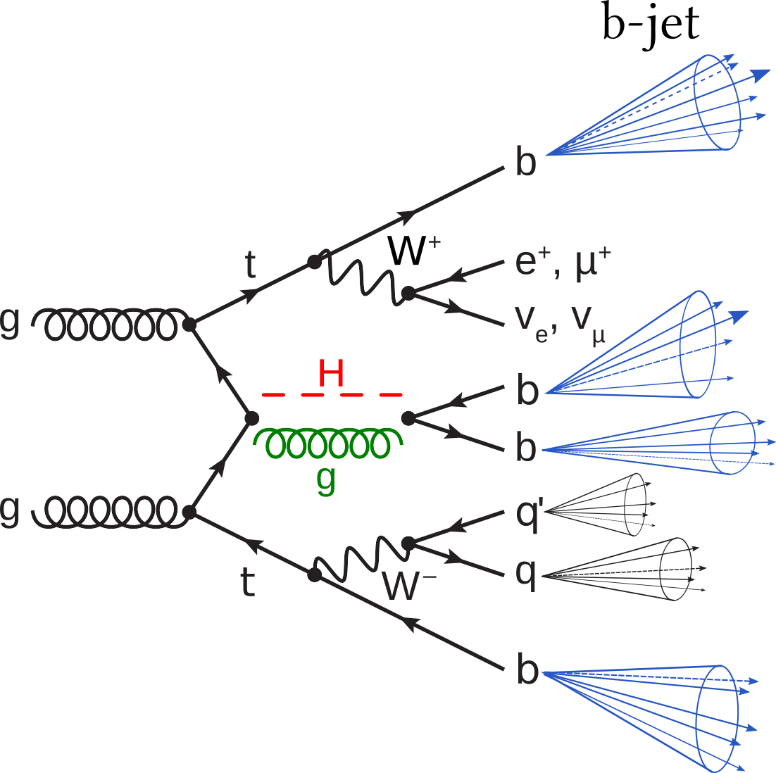
^{The Feynman diagram of the process of interest with a depiction of the final state jets, produced by the hadronization of the quarks. With jets coming from the $b$-quarks and the $q$, $q’$ quarks are illustrated using blue and black colour respectively.}

Analysis Features

For the $t\overline{t}H(b\overline{b})$ analysis using the semi-leptonic channel as described in the theory section, we have the following objects:

For the each jet we have 8 features: $(p_T,\,\eta,\,\phi,\,E,\,\text{b-tag},\,p_x,\,p_y,\,p_z)$
For MET we have 4 features: $(p_T,p_x,p_y,\phi)$
For the lepton (electron or muon) we have 7 features: $(p_T,\,\eta,\,\phi,\,E,\,p_x,\,p_y,\,p_z)$

We observed that inputting “redundant” information to our models by providing both Cartesian coordinate and $(p_T,\eta,\phi)$ representation led to better performance in the autoencoder.

Pre-Selection Cuts

In the pre-selection step, we require the electrons and muons to pass selection criteria of the transverse momentum $p_T$, pseudorapidity $\eta$ and isolation with respect to jets. Namely, the object selection cuts are:

$p_T>30$ GeV, $|\eta|<2.1$ and iso $>0.1$ for the electrons
$p_T>26$ GeV, $|\eta|<2.1$ and iso $>0.1$ for the muons
$p_T>30$ GeV, $|\eta|<2.4$ for the jets

After this initial object selection, we further consider events with at least one lepton and at least 4 jets from which at least two are b-tagged. Thus, the following event selection criteria are used: $n^\text{jet}\geq 4,\, n^\text{b-tag}\geq 2\; \text{and}\; n^\text{leptons}=1$

From the leading-order description of the process depicted in the feynman diagram we identify that the nominal expectation consists of 4 b-tagged jets and 2 jets of any flavour, hence 6 jets in total. For our analysis, we keep the 7 most energetic jets of each event, allowing one extra jet to take into account initial or final state radiation. The jets are sorted from highest with index 0, to lowest energetic with index 6. Summarising, the observables in our data are

\[\begin{equation*} \# \text{features} = 8\times 7\, (\text{jets})\, +7\, (1\, \text{lepton})\, +4\, (\text{MET})\, =67\ \label{eq:n_features} \end{equation*}\]

After all the cuts are applied, .npy ntuples for signal and background events, containing the 67 variables, are saved to be further normalized as described on the normalization page.